How To: Explain Why LeBron is Bad at Free Throws

Isolating play by play data with hoopR

Having studied computer science in undergrad, been a consultant for six years, and taken courses like “Whole Brain Communication” in my MBA, I thought I was fairly well versed in how to analyze and present data. This Substack was a way for me to use that skillset toward something I’m passionate about and hoped others would find interesting. Somewhat arrogantly, I did not expect to discover as many “unknown unknowns”, and learn as much as I have in in the last 8 months, but it’s been an awesome bonus. Things like:

• Advanced web scraping 😍🥣

• Creative and impactful stats

• Coding techniques, mostly in R and Python

  • Including using the wehoop and hoopR packages, for things like play-by-play data, game logs, player photos, and more

• Data visualization tools & techniques (s/o Datawrapper, Flourish, ggplot & Manim)

I’ve also compiled some big datasets relating to names, trade networks, instagram proclivities, and the evolving level of happiness in every major US city (coming soon!).

Some of you may find these things valuable, whether you want to recreate my findings for a different player or time period, leverage a specific piece of the process, or are just curious! So, starting today, I’ll be sharing some of the technical specifics behind the scenes of my stories. Let me know if there’s anything you’ve seen on here you want to learn more about.

To start off, here’s the process I went through to explore the question:

Why is LeBron Bad at Free Throws?

This analysis appeared as a postscript to What If Free Throws were Free? In that piece I wrote,

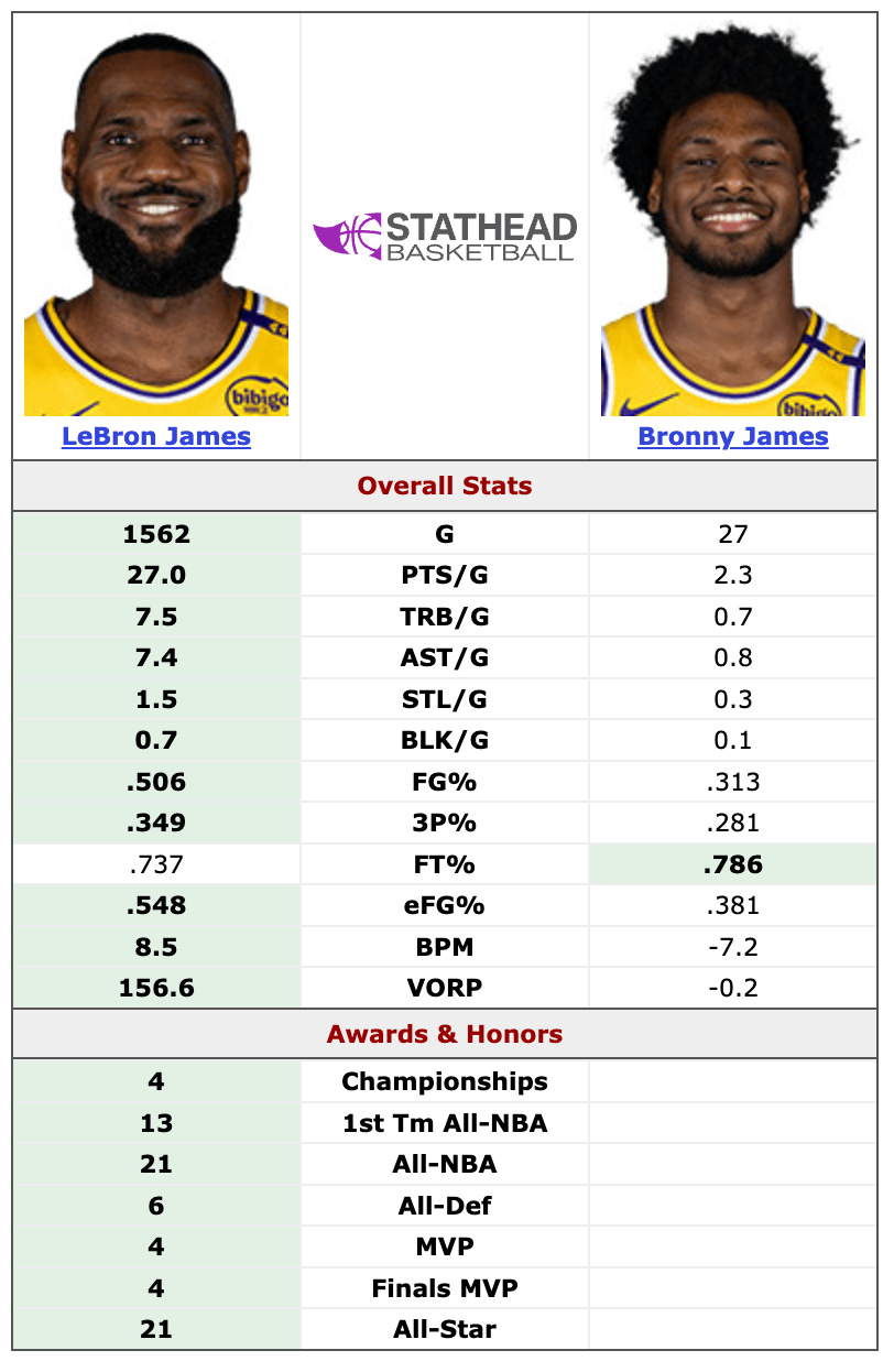
In any given season LeBron James has made between 67% and 78% of his free throws. That’s certainly not DeAndre Jordan levels of struggle from the line, but it’s not great. For someone who puts a ridiculous amount of time, effort, and money into optimizing every part of his game, you’d think he’d have been able to figure out free throw shooting at some point in the last two decades. It’s one of the most isolated, easy-to-practice events in basketball.

I also noted what makes a free throw unique, including that you usually get multiple attempts from the exact same spot over the course of the game and can take all the time you need to catch your breath before shooting, two things I ultimately concluded don’t help LeBron at the line.

To get there, I needed to pull every single free throw LeBron has taken in his career, all 11,735 of them.¹ We can use the hoopR package for this.²

First, we get all of his games:³,⁴

library(dplyr)
library(hoopR)

#Get LeBron (player_id 2544)'s Game Logs
lebron_id = '2544'
lebron_games_2025 <- nba_playergamelogs(player_id = lebron_id, season = '2024-25')$PlayerGameLog
lebron_games_2024 <- nba_playergamelogs(player_id = lebron_id, season = '2023-24')$PlayerGameLog
lebron_games_2023 <- nba_playergamelogs(player_id = lebron_id, season = '2022-23')$PlayerGameLog
lebron_games_2022 <- nba_playergamelogs(player_id = lebron_id, season = '2021-22')$PlayerGameLog
lebron_games_2021 <- nba_playergamelogs(player_id = lebron_id, season = '2020-21')$PlayerGameLog
lebron_games_2020 <- nba_playergamelogs(player_id = lebron_id, season = '2019-20')$PlayerGameLog
lebron_games_2019 <- nba_playergamelogs(player_id = lebron_id, season = '2018-19')$PlayerGameLog
lebron_games_2018 <- nba_playergamelogs(player_id = lebron_id, season = '2017-18')$PlayerGameLog
lebron_games_2017 <- nba_playergamelogs(player_id = lebron_id, season = '2016-17')$PlayerGameLog
lebron_games_2016 <- nba_playergamelogs(player_id = lebron_id, season = '2015-16')$PlayerGameLog
lebron_games_2015 <- nba_playergamelogs(player_id = lebron_id, season = '2014-15')$PlayerGameLog
lebron_games_2014 <- nba_playergamelogs(player_id = lebron_id, season = '2013-14')$PlayerGameLog
lebron_games_2013 <- nba_playergamelogs(player_id = lebron_id, season = '2012-13')$PlayerGameLog
lebron_games_2012 <- nba_playergamelogs(player_id = lebron_id, season = '2011-12')$PlayerGameLog
lebron_games_2011 <- nba_playergamelogs(player_id = lebron_id, season = '2010-11')$PlayerGameLog
lebron_games_2010 <- nba_playergamelogs(player_id = lebron_id, season = '2009-10')$PlayerGameLog
lebron_games_2009 <- nba_playergamelogs(player_id = lebron_id, season = '2008-09')$PlayerGameLog
lebron_games_2008 <- nba_playergamelogs(player_id = lebron_id, season = '2007-08')$PlayerGameLog
lebron_games_2007 <- nba_playergamelogs(player_id = lebron_id, season = '2006-07')$PlayerGameLog
lebron_games_2006 <- nba_playergamelogs(player_id = lebron_id, season = '2005-06')$PlayerGameLog
lebron_games_2005 <- nba_playergamelogs(player_id = lebron_id, season = '2004-05')$PlayerGameLog
lebron_games_2004 <- nba_playergamelogs(player_id = lebron_id, season = '2003-04')$PlayerGameLog

# Combine games from each season into a single dataframe
lebron_games <- rbind(lebron_games_2025, lebron_games_2024, lebron_games_2023, lebron_games_2022, lebron_games_2021, lebron_games_2020, lebron_games_2019, lebron_games_2018, lebron_games_2017, lebron_games_2016, lebron_games_2015, lebron_games_2014, lebron_games_2013, lebron_games_2012, lebron_games_2011, lebron_games_2010, lebron_games_2009, lebron_games_2008, lebron_games_2007, lebron_games_2006, lebron_games_2005, lebron_games_2004)

Once we have all of the game information, we can use the unique set of game identifiers to get the data for every play using nba_pbps() from hoopR:⁵

# Get unique game IDs
lebron_games <- lebron_games %>%
  select(GAME_ID) %>%
  distinct()
lebron_games <- lebron_games$GAME_ID

# Get play-by-play data for every game
lebron_pbps <- nba_pbps(game_ids = lebron_games, version = 'v2')

Then we can filter down to just LeBron’s free throws (event_type 3):

#Filter for LeBron FTs
lebron_FTs <- lebron_pbps %>% 
  filter(
    player1_id == lebron_id,
    event_type == 3
  )

This should leave you with 11,735 rows, the number of free throws LeBron has attempted over his career through the 2024-25 season. Next we need to categorize those attempts as makes or misses. This is captured in the description columns, which are unhelpfully separated into ‘home_description’ for plays by the home team and ‘visitor_description’ for plays by the away team. We can, however, simply combine those into a single description:

#Combine home and away
lebron_FTs <- lebron_FTs %>% 
  mutate(description = ifelse(is.na(home_description), visitor_description, home_description))

Then we use that to categorize makes (1) and misses (0):⁶

#Categorize makes vs misses
lebron_FTs <- lebron_FTs %>% 
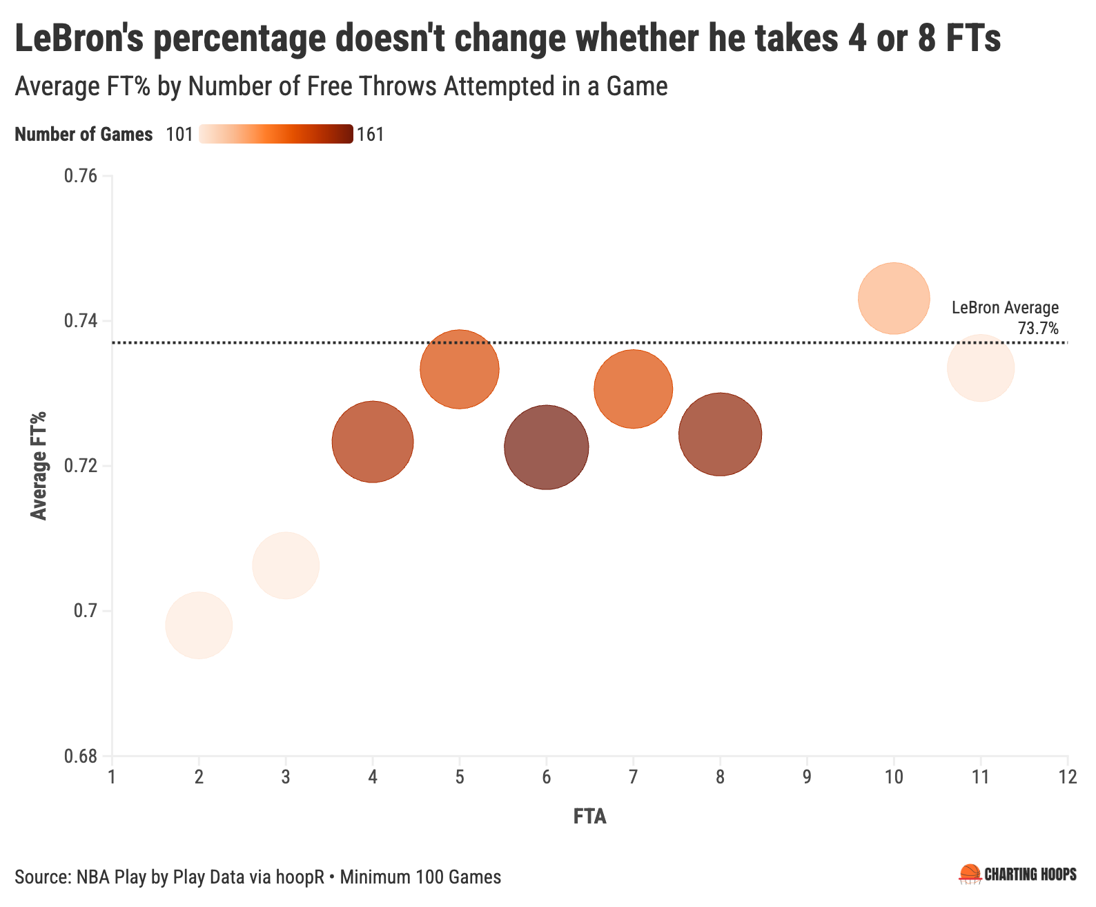
  mutate(Make = ifelse(startsWith(description, “MISS”), 0, 1))

Now we can start doing some analysis. First up, free throw percentage by number of attempts in the game.

I create a helper dataframe that summarizes free throws made (FTM), free throws attempted (FTA), and free throw percentage (FT.) for each game:

fts_per_game <- lebron_FTs %>% 
  group_by(game_id) %>% 
  summarize(FTA = n(), #Count of all rows
            FTM = sum(Make),
            FT. = FTM/FTA
            )

Then I use that to calculate LeBron’s average free throw percentages in games where he takes [X] number of free throws using the group_by() function:

#FT% by FTA
fts_per_game_data <- fts_per_game %>% 
  group_by(FTA) %>% 
  summarize(n = n(), #Number of games with this # of FTAs
            avg_FT. = mean(FT.) #Average FT% in those games
            ) %>% 
  filter(n >= 100) #Exclude FTs from FTAs taken in fewer than 100 games

We can then plot this in a basic column chart using ggplot or, do what I did, export it to a CSV, upload that to Flourish, and design the bubble chart there.

fts_per_game_data %>% 
  ggplot(aes(x = factor(FTA), y = avg_FT.)) +
  geom_col(fill = "#ff6e2a") +
  labs(x = “Free Throw Attempt (FTA)”, y = “Free Throw %”, title = “Mean FT% by FTAs”) +
  theme_minimal()

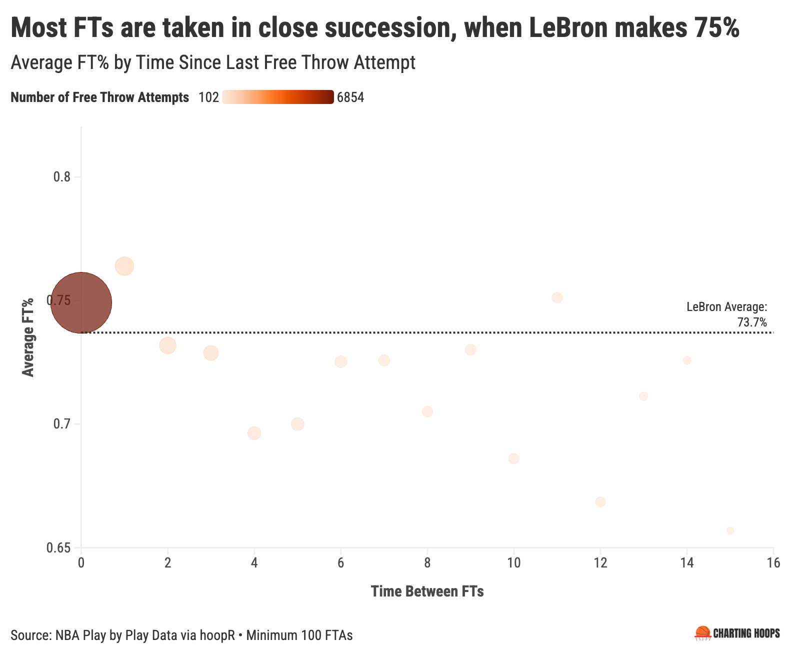
write.csv(fts_per_game_data, “fts_per_game_data.csv”)

Next up, I looked into how LeBron’s free throw percentage changed based on how long it had beed since his last attempt.

This required the extra step of tracking how far into the game we were. In the play by play data. I decided to use game time, though you could use real time with the ‘minute_game’ column as well. To calculate the amount of game time that is elapsed we can do some math on the time remaining in a quarter, knowing an NBA quarter is 12 minutes long. Do this back on the full lebron_pbps dataframe, before filtering to just the free throws.

#Track minutes into game
lebron_pbps <- lebron_pbps %>% 
  mutate(game_time_elapsed = ((period - 1) * 12) + (12 - minute_remaining_quarter - (seconds_remaining_quarter/60)))

Then re-filter to just free throws, and in our lebron_FTs dataframe we can count the time since the last play (which is, by definition, a LeBron free throw since we’ve filtered to only those plays) using the lag function, which takes the variable from the previous row:⁷

lebron_FTs <- lebron_FTs %>%
  arrange(game_id, game_time_elapsed) %>%
  group_by(game_id) %>%
  mutate(
    time_since_last_play = game_time_elapsed - lag(game_time_elapsed, default = first(game_time_elapsed)) 
  ) %>%
  ungroup()

Then we can follow the same process as before to look at free throw percentage by time_since_last_play, with the small added step of grouping the times to the nearest, rounded down minute:

#Group minutes
lebron_FTs <- lebron_FTs %>% 
  mutate(time_since_last_play = floor(time_since_last_play))

#FT% by Time Since Last FT
fts_by_time_since_FT <- lebron_FTs %>% 
  group_by(time_since_last_play) %>% 
  summarize(FTA = n(),
            FTM = sum(Make),
            FT. = FTM/FTA
            ) %>% 
  filter(FTA >= 100) #Exclude FTs from breaks taken in fewer than 100 games
  
write.csv(fts_by_time_since_FT, “fts_by_time_since_FT.csv”)

#FT% by Time Remaining Chart
fts_by_time_since_FT %>% 
  ggplot(aes(x = factor(time_since_last_play), y = FT.)) +
  geom_col(fill = “#ff6e2a”) +
  labs(x = “Minutes Since Last FT”, y = “Free Throw %”, title = “Mean FT% by Minutes Since Last FT”) +
  theme_minimal()

As expected, we see that most of the free throw attempts come within 0 minutes of the last one, since you usually get two free throw attempts at once.

Finally, let’s look at LeBron’s splits by how many minutes he’s played.

Again, this requires one extra data creation step on the full lebron_pbps dataframe, namely tracking how many minutes LeBron has played so far in a given game, up to a given play.

The play by play data includes information on the 10 players on the court, by listing each player’s player_id in one of 10 columns named away_player1 … away_player5 and home_player1 … homeplayer5. So for every play we can check if LeBron was on the court.

Then, using the game_time_elapsed variable created above we can track the amount of time that passed between each play.

Finally we isolate the plays when LeBron was on the court and track a running, cumulative summation of those minutes.

#Calculate LeBron MP in game up to given play
lebron_pbps <- lebron_pbps %>%
  # Rowwise lets you check LeBron’s presence in each play
  rowwise() %>%
  mutate(
    lebron_on_court = any(pick(starts_with(”away_player”), starts_with(”home_player”)) == lebron_id)
  ) %>%
  ungroup() %>%
  arrange(game_id, game_time_elapsed) %>% # Ensure data sorted by game and earliest-to-latest
  group_by(game_id) %>%
  mutate(

    # For each play, get difference in minutes to next play (previous playtime - current playtime)
    play_interval = game_time_elapsed - lag(game_time_elapsed, default = first(game_time_elapsed)),
    # On the very first row per game, interval should be 0
    play_interval = ifelse(row_number() == 1, 0, play_interval),

    # Only count interval if LeBron is on court for that interval
    lebron_mins_in_play = ifelse(lag(lebron_on_court, default = first(lebron_on_court)), play_interval, 0),
    # Cumulative sum: total LeBron minutes up to this play
    lebron_game_mins = cumsum(lebron_mins_in_play)
  ) %>%
  ungroup()

We’re in the clear. Final step is to repeat the same process from the prior to charts.

#Group minutes
lebron_FTs <- lebron_FTs %>% 
  mutate(lebron_game_mins = floor(lebron_game_mins))

fts_by_mp <- lebron_FTs %>% 
  group_by(lebron_game_mins) %>% 
  summarize(FTA = n(),
            FTM = sum(Make),
            FT. = FTM/FTA
            ) %>% 
  filter(FTA >= 100)

write.csv(fts_by_mp, “fts_by_mp.csv”)

#FT% by Time Remaining
fts_by_mp %>% 
  ggplot(aes(x = factor(lebron_game_mins), y = FT.)) +
  geom_col(fill = “#ff6e2a”) +
  labs(x = “Minutes Played”, y = “Free Throw %”, title = “Mean FT% by Minutes Played”) +
  theme_minimal()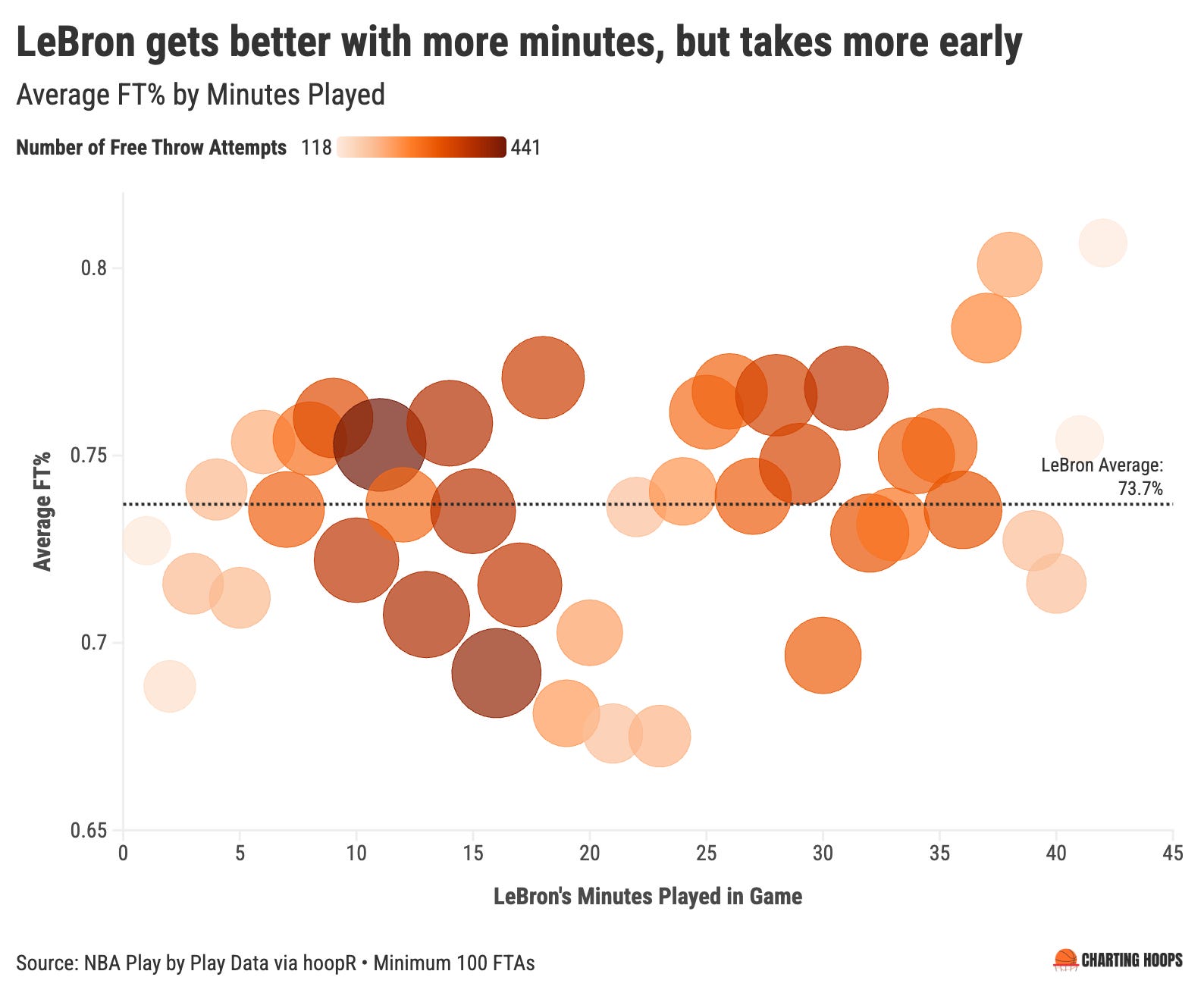

And there you have it. Hope this was helpful for understanding how to get information for specific plays (all the way back to 22 years ago no less), and work with certain features of it (time and players on in this case). I’ll certainly be covering a lot more of the things that are possible with this level of granularity in the future. Stay tuned!

---

1. Regular season only.

2. If you haven’t used hoopR before you’ll need to install it with install.packages(“hoopR”).

3. hoopR can be finicky when trying to pull too much data at once, so splitting up this run by season seems to increase the reliability. Once you combine all the season dataframes, there should be 1,562 rows, matching LeBron’s regular season games played through 2024-25.

4. You can see the full list of player ids (PERSON_ID) using the nba_commonallplayers() hoopR function.

5. Note: This talks a few minutes to run. LeBron had been in a LOOOOOOOOOOT of plays.

6. For what it’s worth, if you want to check as you go you can copy and paste the game ID + “NBA game” into Google and it usually pulls up the NBA page for that game, where you can visually inspect the play-by-play yourself.

7. If it’s LeBron’s first free throw of the game, time_since_last_play should be equal to game_time_elapsed.